Analysis of Movie Ratings Using IMDB Data
Summary of the Project
Import and inspect the IMDB dataset using skimr and dplyr package functions.
Clean the data set and conduct exploratory data analysis (EDA).
Use ggplot2 package functions to visualize relationships between variables of interest. We want to investigate the relationship between gross earnings in the US box office [gross] and the number of facebook likes cast members received [likes], IMDB average rating [ratings] and the movie’s budget [budget] respectively.
An investigation into whether the mean IMDB ratings for movie director Steven Spielberg and Tim Burton are the same or not.
Importing and Inspecting the IMDB Dataset
We looked at a subset sample of movies, taken from the Kaggle IMDB 5000 movie dataset
movies <- read_csv(here::here("movies.csv"))
glimpse(movies)
## Rows: 2,961
## Columns: 11
## $ title <chr> "Avatar", "Titanic", "Jurassic World", "The Avenge…
## $ genre <chr> "Action", "Drama", "Action", "Action", "Action", "…
## $ director <chr> "James Cameron", "James Cameron", "Colin Trevorrow…
## $ year <dbl> 2009, 1997, 2015, 2012, 2008, 1999, 1977, 2015, 20…
## $ duration <dbl> 178, 194, 124, 173, 152, 136, 125, 141, 164, 93, 1…
## $ gross <dbl> 7.61e+08, 6.59e+08, 6.52e+08, 6.23e+08, 5.33e+08, …
## $ budget <dbl> 2.37e+08, 2.00e+08, 1.50e+08, 2.20e+08, 1.85e+08, …
## $ cast_facebook_likes <dbl> 4834, 45223, 8458, 87697, 57802, 37723, 13485, 920…
## $ votes <dbl> 886204, 793059, 418214, 995415, 1676169, 534658, 9…
## $ reviews <dbl> 3777, 2843, 1934, 2425, 5312, 3917, 1752, 1752, 35…
## $ rating <dbl> 7.9, 7.7, 7.0, 8.1, 9.0, 6.5, 8.7, 7.5, 8.5, 7.2, …skim(movies)| Name | movies |
| Number of rows | 2961 |
| Number of columns | 11 |
| _______________________ | |
| Column type frequency: | |
| character | 3 |
| numeric | 8 |
| ________________________ | |
| Group variables | None |
Variable type: character
| skim_variable | n_missing | complete_rate | min | max | empty | n_unique | whitespace |
|---|---|---|---|---|---|---|---|
| title | 0 | 1 | 1 | 83 | 0 | 2907 | 0 |
| genre | 0 | 1 | 5 | 11 | 0 | 17 | 0 |
| director | 0 | 1 | 3 | 32 | 0 | 1366 | 0 |
Variable type: numeric
| skim_variable | n_missing | complete_rate | mean | sd | p0 | p25 | p50 | p75 | p100 | hist |
|---|---|---|---|---|---|---|---|---|---|---|
| year | 0 | 1 | 2.00e+03 | 9.95e+00 | 1920.0 | 2.00e+03 | 2.00e+03 | 2.01e+03 | 2.02e+03 | ▁▁▁▂▇ |
| duration | 0 | 1 | 1.10e+02 | 2.22e+01 | 37.0 | 9.50e+01 | 1.06e+02 | 1.19e+02 | 3.30e+02 | ▃▇▁▁▁ |
| gross | 0 | 1 | 5.81e+07 | 7.25e+07 | 703.0 | 1.23e+07 | 3.47e+07 | 7.56e+07 | 7.61e+08 | ▇▁▁▁▁ |
| budget | 0 | 1 | 4.06e+07 | 4.37e+07 | 218.0 | 1.10e+07 | 2.60e+07 | 5.50e+07 | 3.00e+08 | ▇▂▁▁▁ |
| cast_facebook_likes | 0 | 1 | 1.24e+04 | 2.05e+04 | 0.0 | 2.24e+03 | 4.60e+03 | 1.69e+04 | 6.57e+05 | ▇▁▁▁▁ |
| votes | 0 | 1 | 1.09e+05 | 1.58e+05 | 5.0 | 1.99e+04 | 5.57e+04 | 1.33e+05 | 1.69e+06 | ▇▁▁▁▁ |
| reviews | 0 | 1 | 5.03e+02 | 4.94e+02 | 2.0 | 1.99e+02 | 3.64e+02 | 6.31e+02 | 5.31e+03 | ▇▁▁▁▁ |
| rating | 0 | 1 | 6.39e+00 | 1.05e+00 | 1.6 | 5.80e+00 | 6.50e+00 | 7.10e+00 | 9.30e+00 | ▁▁▆▇▁ |
Besides the obvious variables of title, genre, director, year, and duration, the rest of the variables are as follows:
gross: The gross earnings in the US box office, not adjusted for inflationbudget: The movie’s budgetcast_facebook_likes: the number of facebook likes cast members receivedvotes: the number of people who voted for (or rated) the movie in IMDBreviews: the number of reviews for that movierating: IMDB average rating
Data Cleaning
Firstly, check for missing values and duplicated entries. There is no missing values, if we use is.na(movies) to check. There are 54 duplicate entries.
Make a table with the count of movies by genre, ranked in descending order
count_of_movies_by_genre <- movies %>%
  group_by(genre) %>%
  count(genre) %>%
  arrange(desc(n))
count_of_movies_by_genre
## # A tibble: 17 × 2 ## # Groups: genre [17] ## genre n ## <chr> <int> ## 1 Comedy 848 ## 2 Action 738 ## 3 Drama 498 ## 4 Adventure 288 ## 5 Crime 202 ## 6 Biography 135 ## 7 Horror 131 ## 8 Animation 35 ## 9 Fantasy 28 ## 10 Documentary 25 ## 11 Mystery 16 ## 12 Sci-Fi 7 ## 13 Family 3 ## 14 Musical 2 ## 15 Romance 2 ## 16 Western 2 ## 17 Thriller 1Produce a table with the average gross earning and budget (
grossandbudget) by genre. Calculate a variablereturn_on_budgetwhich shows how many $ did a movie make at the box office for each $ of its budget. Ranked genres by thisreturn_on_budgetin descending order# producing the new table avg_gross_budget_by_genre <- movies %>% group_by(genre) %>% summarise(avg_gross = mean(gross), avg_budget = mean(budget)) # calculating return_on_budget return_on_budget <- avg_gross_budget_by_genre %>% mutate(return_on_budget = avg_gross/avg_budget) %>% select(genre, return_on_budget) %>% arrange(desc(return_on_budget))Produce a table that shows the top 15 directors who have created the highest gross revenue in the box office. Showing the total gross amount, as well as the mean, median, and standard deviation per director.
movies %>%
  group_by(director) %>%
  summarise(gross_rev = sum(gross), mean_rev = mean(gross), median_rev = median(gross), SD_rev = sd(gross)) %>%
  slice_max(n=15,order_by=gross_rev)
## # A tibble: 15 × 5 ## director gross_rev mean_rev median_rev SD_rev ## <chr> <dbl> <dbl> <dbl> <dbl> ## 1 Steven Spielberg 4014061704 174524422. 164435221 101421051. ## 2 Michael Bay 2231242537 171634041. 138396624 127161579. ## 3 Tim Burton 2071275480 129454718. 76519172 108726924. ## 4 Sam Raimi 2014600898 201460090. 234903076 162126632. ## 5 James Cameron 1909725910 318287652. 175562880. 309171337. ## 6 Christopher Nolan 1813227576 226653447 196667606. 187224133. ## 7 George Lucas 1741418480 348283696 380262555 146193880. ## 8 Robert Zemeckis 1619309108 124562239. 100853835 91300279. ## 9 Clint Eastwood 1378321100 72543216. 46700000 75487408. ## 10 Francis Lawrence 1358501971 271700394. 281666058 135437020. ## 11 Ron Howard 1335988092 111332341 101587923 81933761. ## 12 Gore Verbinski 1329600995 189942999. 123207194 154473822. ## 13 Andrew Adamson 1137446920 284361730 279680930. 120895765. ## 14 Shawn Levy 1129750988 102704635. 85463309 65484773. ## 15 Ridley Scott 1128857598 80632686. 47775715 68812285.Finally, ratings. Produce a table that describes how ratings are distributed by genre. Find the mean, min, max, median, SD and draw a graph to show how ratings are distributed.
ratings_table <- movies %>%
  group_by(genre) %>%
  summarise(mean=mean(rating), min=min(rating), max=max(rating), median=median(rating),SD=sd(rating))

# density graph of rating distribution
ggplot(movies) +
  aes(x=rating, colour = genre) +
  geom_density(size = 1.3) +
  facet_wrap(~genre) +
  theme_bw(base_size = 18) +
  labs(title = "Distribution of IMDB Ratings by Film Genre ",
       x = NULL,
       y = NULL,
       caption = "Source: Kaggle IMDB 5000 Movie Dataset") +
   theme(legend.position = "NONE")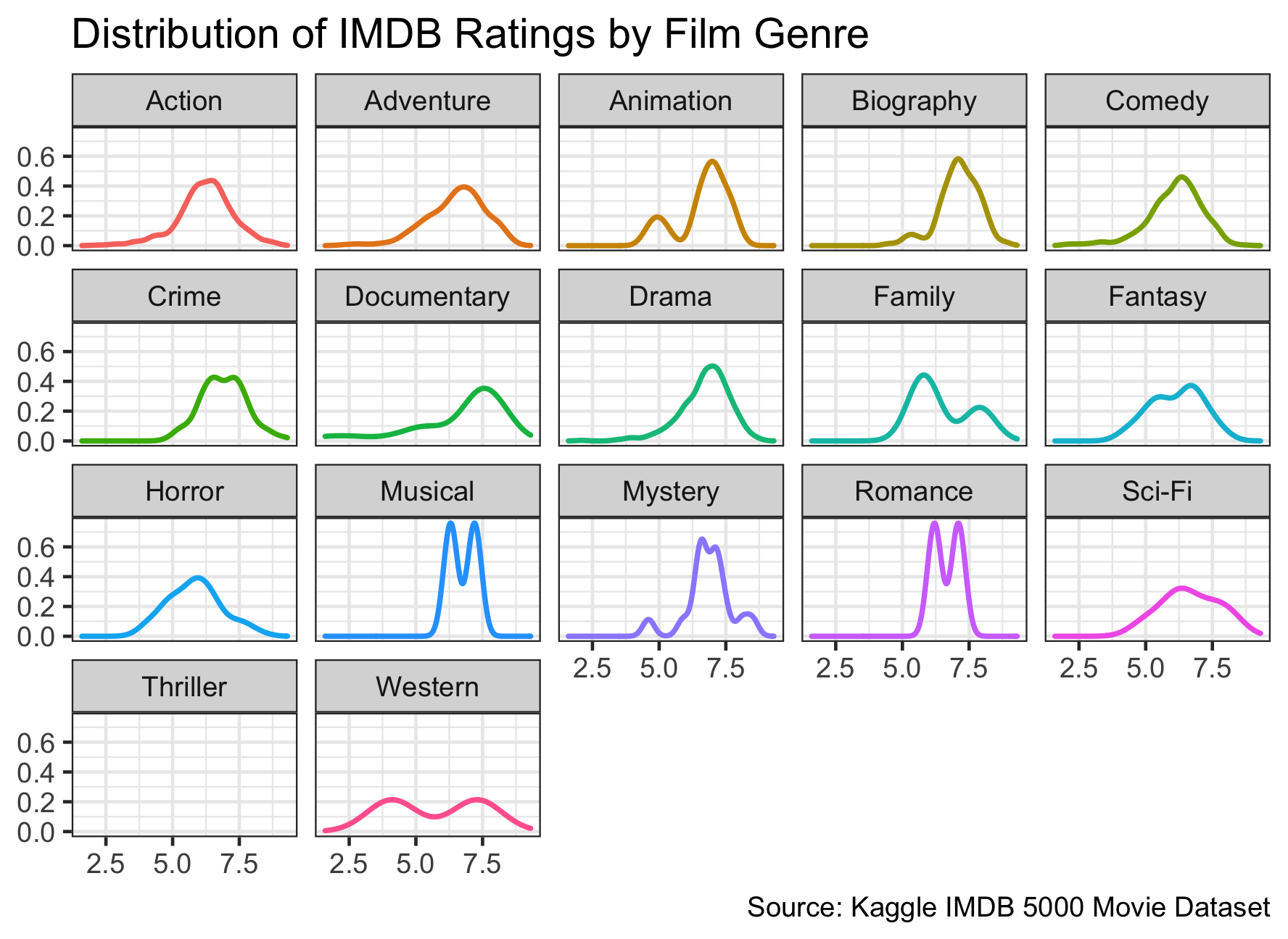
Examine the Relationship of Variables of Interest
- Examine the relationship between
grossandcast_facebook_likes. - The scatter plot below shows that there is a slight positive correlation between ‘gross’ and ‘cast_facebook_like’, although there exist many outliers, such as when likes is less than 100. Therefore, the cast is not likely to be a good predictor. However, many data points lies outside the a line of best fit, therefore, we cannot say with good confidence that it is a good predictor.
ggplot(movies) +
  aes(x = cast_facebook_likes, y = gross) +
  geom_point(size=3) +
  geom_smooth(method='lm') +
  labs (title = "Relationship Between 'gross' and 'cast_facebook_likes'",
        x = "Number of Likes for Cast on Faceboook",
        y = "Gross Earnings in the US Box Office",
        caption = "Source: Kaggle IMDB 5000 Movie Dataset") +
  theme_classic(base_size = 18) +
  scale_x_log10()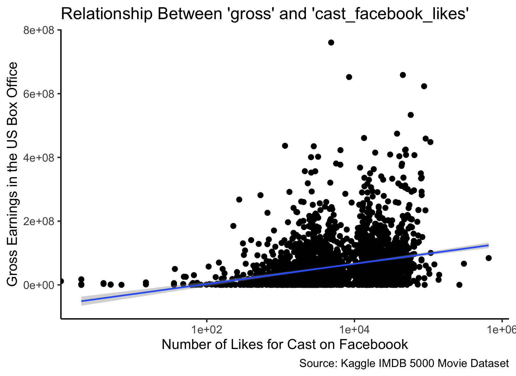
- Examine the relationship between
grossandbudget. - Budget appears to be a good predictor of gross, since the graph shows a positive correlation. Although when the budget is less than 1 million dollars, it is not a good predictor.
ggplot(movies) +
  aes(x=budget, y=gross) +
  geom_point(size =3) +
  geom_smooth(method='lm', se=FALSE) +
  scale_x_log10() +
  labs(title = "Relationship Between 'gross' and 'budget'",
        x = "The Movie's Budget",
        y = "Gross Earnings in the US Box Office",
        caption = "Source: Kaggle IMDB 5000 Movie Dataset") +
  theme_bw(base_size=18)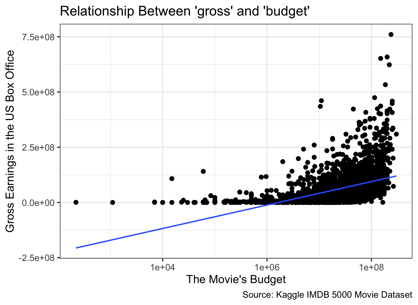
- Examine the relationship between
grossandrating. - Generally, some genre have much more rating than others,for instance, crime, documentary, and mystery. The others, however, have significantly less reviews. For those with high numbers of reviews, such as Action, Adventure, there exist positive correlation between gross and rating which makes IMDB rating a good predictor for those movies.
ggplot(movies) +
  aes(x=rating, y=gross, colour = genre) +
  geom_point(size=2) +
  facet_wrap(~genre) +
  labs(title = 'Relationship Between Rating and Gross Revenue By Genre' ,
       x = NULL,
       y = NULL,
       caption = "Source: Kaggle IMDB 5000 Movie Dataset") +
  theme_bw(base_size=18) +
theme(legend.position = "none") 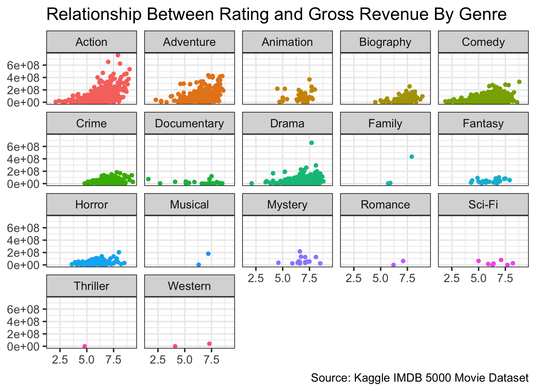
Differences Between the Mean IMDB Ratings for Steven Spielberg and Tim Burton
Null Hypothesis: IMDB mean rating is the same for SS and TB. difference in m =0 Alternative hypothesis: difference in mean is not equal to 0. t-stat: difference between mean divided by standard error p-value
movies <- read_csv(here::here("data", "movies.csv"))
#glimpse(movies)

movies_2 <- movies %>%
  group_by(director) %>%
  filter(director %in% c("Steven Spielberg","Tim Burton")) %>%
  summarise(rating,mean_rating = mean(rating), #find datapoints needed for t distribution.
         sd_rating = sd(rating),
         count=n(),
         t_critical =qt(0.975,count-1),
         se_rating = sd(rating)/sqrt(count),
         margin_of_error = t_critical*se_rating,
         rating_low = mean_rating - margin_of_error,
         rating_high = mean_rating +margin_of_error,
         highest_rating =max(rating),
         lowest_rating = min(rating))

#movies_mean<-count(movies, mean_rating)
#movies_mean
movies_2
## # A tibble: 39 × 12
## # Groups: director [2]
## director rating mean_…¹ sd_ra…² count t_cri…³ se_ra…⁴ margi…⁵ ratin…⁶ ratin…⁷
## <chr> <dbl> <dbl> <dbl> <int> <dbl> <dbl> <dbl> <dbl> <dbl>
## 1 Steven … 7.9 7.57 0.695 23 2.07 0.145 0.301 7.27 7.87
## 2 Steven … 8.1 7.57 0.695 23 2.07 0.145 0.301 7.27 7.87
## 3 Steven … 6.2 7.57 0.695 23 2.07 0.145 0.301 7.27 7.87
## 4 Steven … 8 7.57 0.695 23 2.07 0.145 0.301 7.27 7.87
## 5 Steven … 8.5 7.57 0.695 23 2.07 0.145 0.301 7.27 7.87
## 6 Steven … 6.5 7.57 0.695 23 2.07 0.145 0.301 7.27 7.87
## 7 Steven … 6.5 7.57 0.695 23 2.07 0.145 0.301 7.27 7.87
## 8 Steven … 8.6 7.57 0.695 23 2.07 0.145 0.301 7.27 7.87
## 9 Steven … 8.3 7.57 0.695 23 2.07 0.145 0.301 7.27 7.87
## 10 Steven … 7.4 7.57 0.695 23 2.07 0.145 0.301 7.27 7.87
## # … with 29 more rows, 2 more variables: highest_rating <dbl>,
## # lowest_rating <dbl>, and abbreviated variable names ¹mean_rating,
## # ²sd_rating, ³t_critical, ⁴se_rating, ⁵margin_of_error, ⁶rating_low,
## # ⁷rating_high ggplot(movies_2, aes(x = mean_rating,y = director))+
geom_point() +
geom_errorbar(data = movies_2,aes(xmin = rating_low, xmax=rating_high,height=0.2), size = 1, height = 0.1) +
labs(x = "Mean IMDB Rating",
y = NULL,
title = "Mean IMDB Rating for Spielburg and Burton",
subtitle="95% confidence interval overlap") +
geom_rect(aes(xmin=7.27, xmax= 7.33, ymin=0, ymax=3),
fill = "grey70",
alpha = 0.5)+
theme_minimal(base_size = 16) #+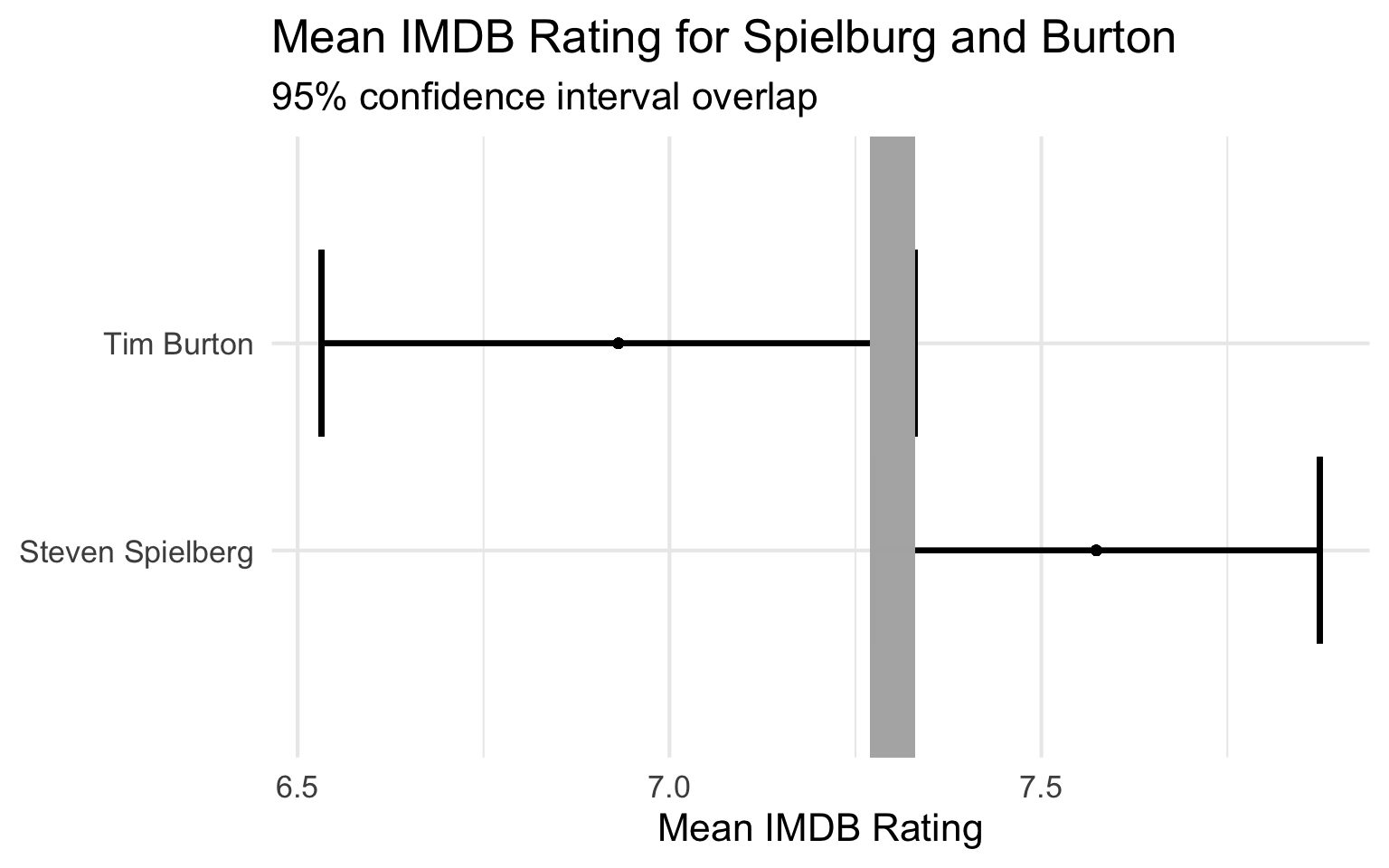
  #geom_text(aes(x= mean_rating, label = labels), vjust=0, nudge_y =0.05,overlap=FALSE) +
  #geom_text(label=mean)
  #theme_bw()
As there is an overlap in the confidence interval, we will now need to use t test for further examination
With a p-value of 1%<5%, we can reject the null hypothesis that Spielburg and Burton have the same mean rating.
We should use both the
t.testcommand and theinferpackage to simulate from a null distribution, where you assume zero difference between the two.By using the infer package, we can simulate from a null distribution and compute p-values (with get_p_value()). As seen below, the p-value from the null distribution gives 0.4%<1%<5%. Thus, we can infer that the null hypothesis can be rejected.
We can conclude that the difference in mean ratings for the two directors is unlikely to be zero.
t.test(rating~director, data = movies_2) #find t-stat, p-value##
## Welch Two Sample t-test
##
## data: rating by director
## t = 3, df = 31, p-value = 0.01
## alternative hypothesis: true difference in means between group Steven Spielberg and group Tim Burton is not equal to 0
## 95 percent confidence interval:
## 0.16 1.13
## sample estimates:
## mean in group Steven Spielberg mean in group Tim Burton
## 7.57 6.93#simulating a null world using infer()
set.seed(1234)
ratings_in_null_world <- movies_2 %>%
specify(rating~director) %>% # we want to look at ratings of directors
hypothesize(null = "independence") %>% # hypothesize that the difference is 0
generate(reps=1000, type="permute") %>% # create a bunch of simulated samples
calculate(stat="diff in means", order = c("Steven Spielberg","Tim Burton")) # find difference in means of each sample.
#ratings_in_null_world visualize, with shaded p value
ratings_in_null_world %>%
visualize() +
shade_p_value(obs_stat = 0.64, direction = "two-sided")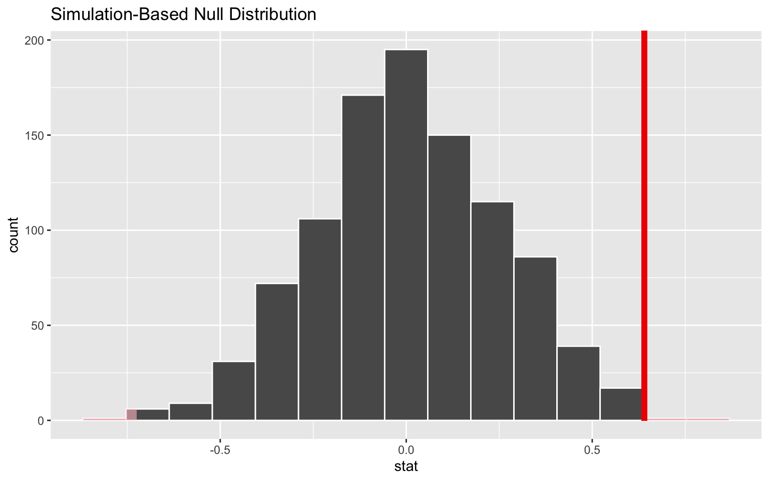
# finding p-value of simulated distribution
p_value <- ratings_in_null_world%>%
  get_p_value(obs_stat = .64, direction = "two-sided")
p_value
## # A tibble: 1 × 1
## p_value
## <dbl>
## 1 0.004